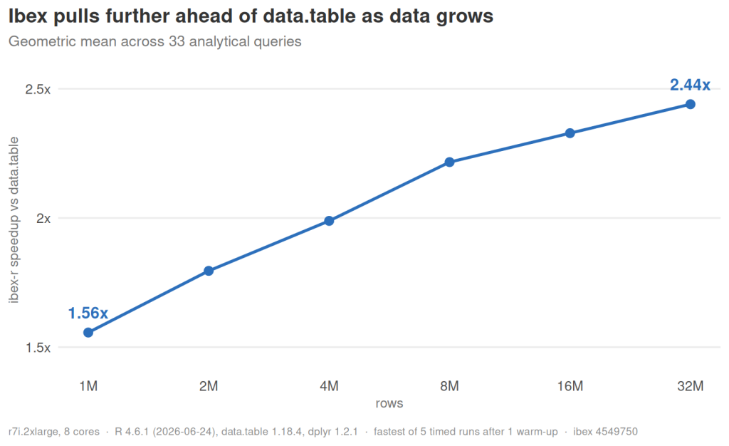
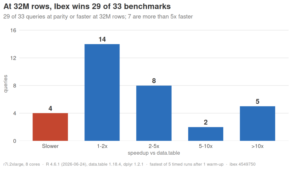
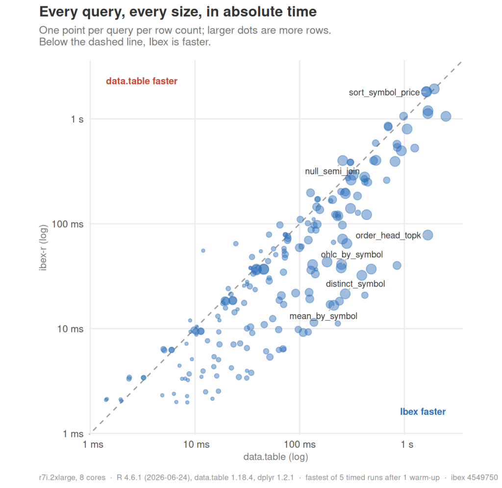
The R Ibex package brings the Ibex query engine to R by providing a dplyr-compatible backend. Ibex can also be used as a standalone language through a REPL, notebooks or compiled to C++. The R Ibex package is significantly faster than dplyr and faster (more than an order of magnitude faster in 5/33 tests) than data.table on the majority of tasks benchmarked. The performance gap grows with data size. The script is in the repo and the paired results per task are in the final plot.
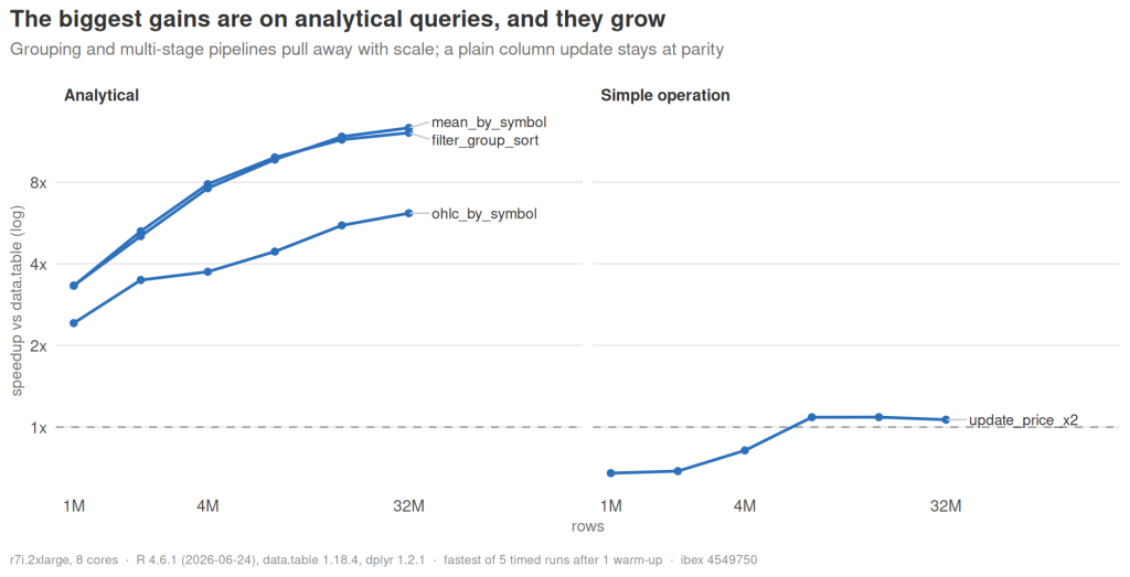
Ibex mainly wins on analytical queries and remains competitive on simple data updating operations. Ibex is still in development so further performance gains are on the cards. For the specific queries for which Ibex is slower, I’m aiming for parity, on those it might be hard to beet data.table as it is of course quite fast and well-integrated into R. The distribution of speedups and the performance over the benchmarked sizes for various task groups is shown below.
How
The wins are obtained by lazy by default queries and typed data frames, both of which enable algorithmic wins. Ibex uses more space-efficient data structures and has many specializations for specific query shapes. The package avoids interacting with R during query execution which would give all performance gains away again. The results below are from an 8 core, 64GB machine on AWS (r7i.2xlarge).
Algorithmic wins
One example of a win over data.table that Ibex can obtain is the following code: head(dt[order(x)], 100). In this statement, data.table will first sort and then take the top 100 rows, this algorithm is O(n log n) in general. The equivalent Ibex code tbl[order x, head 100] or tbl[order x][head 100] is analyzed before running and an efficient O(n log k) algorithm is employed.
Caveats and plans
This is still an experimental package, there will be bugs and there will be performance regressions. The Ibex package falls back on dplyr if it can’t handle a query.
Mixing queries with arbitrary R functions is not supported well yet. At the moment, I’m looking at efficiently falling back to R vectorized calls during Ibex query execution for functions that are defined in R.
Lazy execution of the queries will allow optimized reading and decoding of parquet files depending on which rows and columns are required, this has been implemented in Ibex proper but the R package does not yet take advantage of this fusion.
All observations
The plot below shows each paired observation of Ibex vs data.table. The performance benefits it gives cover many use cases and can be substantial. For the cases where Ibex loses, the loss is often minimal.
Ibex is a new table focused language for analysis of tabular data and time-series. Its goal is to combine the conciseness of data.table with speed, obtained by native code generation, a fast interpreter and lots of attention for efficient algorithms and code. It aims to make exploratory queries quick to write and fast to execute. The goal is to make data analysis feel smooth and fast. A demo of a quant pipeline gives an idea of what is possible.
Since my previous post on Ibex a lot has happened. Ibex gained useful features, speed and benchmarks (these numbers are before multithreading support) and cross platform binaries. The new features are
Rich join support, with a basic approach to join planning.
Vectorization and efficient algorithms of common table operations.
Date and Timestamps are efficiently stored as signed counts since epoch.
Time Series support: windowing, rolling, grouped rolling, resampling, as-of joins.
Fast, vectorized RNG using Zorro (xoshiro256++ based). Purpose-built for Ibex and split off.
Multithreading in active development but for OHLCV analysis I have some promising results already. However, I only looked at this narrow use case of writing.
Some integration work for Python and R but still alpha.
Plugins for I/O and data analytics.
Some exploration in how an effect system can work for Ibex. The syntax supports it but the Ibex optimizer doesn’t use the information yet. Long term goal is to allow Ibex to efficiently use code in plugins, for example by reordering function calls if it can be proven this is correct based on the given effects.
Ergonomics
I started working on Ibex with a focus on ergonomics. It should be easy to write quick analysis without too much special characters or using the shift key. OHLCV looks like this:
ticks[ select {
     open = first(price),
     high = max(price),
     low = min(price),
     close = last(price),
     volume_sum = sum(volume) },
   by symbol,
   resample 10s,
   order symbol ]
Ticks is a table (TimeFrame) with columns timestamp, symbol, price and volume. The expression selects the data it wants in the select clause, by symbol instructs Ibex to group the rows by symbol, resample 10s uses a duration literal to resample the data in 10 second long buckets and the final clause orders by symbol. The ordering by timestamp is implicit. Short, sweet and easy to write. The code is succinct but there is no need to do any code golf to get to that low count. select can be omitted if you want. The syntax borrows heavily from both R’s data.table and SQL keywords. Compared to libraries such as Polars, Pandas and data.table, there is no need to quote column names. The Ibex syntax is specialized for tables and will look up names in the table context first, then in the outer scope. Compared to SQL, the order of the clauses is free so it is possible to write queries in the order that feels natural for the problem at hand. Of course, I’m biased but I would use the Ibex syntax for its convenience alone.
Joins
Joins are easy to write as well, and quite fast. Using the nycflights13 data set we can get the name of the carrier of the flight using a join and then do a group by and count. Very little boilerplate required. Every word or symbol in the expression is contributing something meaningful to the semantics of the query.
The TimeFrame is a unique feature to Ibex. A TimeFrame is like a regular DataFrame that is always has one chosen timestamp column as the final in an ordering. It is what makes the resample keyword in the snippet above work. This simplifies writing time series analysis such as windowing and resampling and reduces the likelihood of errors.
Performance
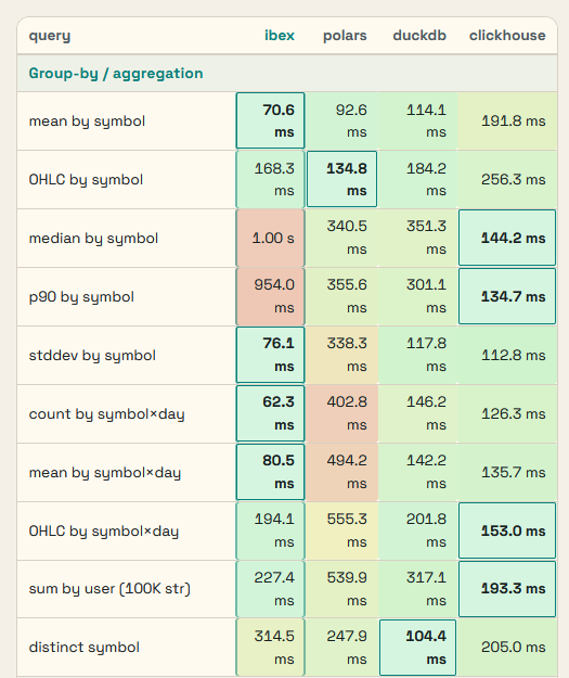
Being convenient might not be enough to convince everybody though. I have done some benchmarking and am still doing more. Ibex performs very well on one core but lags more mature engines when the core count goes up. Often, on a single core it is competitive with multithreaded Polars and now that multithreaded Ibex is in development, I’m confident that it will be be beating Polars, Clickhouse and DuckDB in many real world use cases in the coming months. Fully replicating the PDS benchmark ran by Polars is on the short term roadmap. An excerpt from the in-memory benchmarks, single threaded Ibex against the multithreaded competition (8 cores) on 32 million rows:
Deep dives in why Ibex performs as well as it does will be published in follow-up blog posts.
Plugins and interop
Ibex supports plugins to allow interop and more general programming. Through these plugins Ibex can read and write parquet and CSV. For data analysis, there is a k-means, pca plugin. For generating some fake data, you can use the data_gen plugin:
The important table operations have been implemented and perform quite well on a single core. Improving multithreading support and further development of the plugins. My early experiments have shown that on the small PDS set (SF-1) Ibex is competitive on a single core, it loses when core counts go up. Making Ibex work efficiently on huge machines will take some effort, probably a lot.
Conclusion
Ibex is an ergonomic and fast alternative for the well known analytical data processors such as Polars and DuckDB. In my benchmarking it beats the alternatives on a single core and the syntax is both easy to read and write. Efficient threading is actively being worked on and initial experiments suggest that the single core performance holds up in a multithreaded setting.
Anthropic used a swarm of Claude Opus 4.6 agents to build a C compiler for about $20,000 in API costs with minimal intervention. It did make me realise that while I have been a happy user of R’s data.table for quite some time, the time to build something better is here. Third party packages like data.table but also pandas, Polars, the Tidyverse are bolted on an existing scripting language. These packages are marvels of engineering but the required hacks do have both pros and cons. They can lead to surprising behaviour (often: bugs) and when performance matters, a deep understanding of what happens under the hood is needed. The trade-off seems structural. A language focused on data frames might be a much more powerful tool.
So I, together with my team of LLMs started building a new language. The result is Ibex. It is far from done but it does do some useful work already:
CSV and Parquet reading
Select / Update / Filter / Group / Aggregate
Regular and table variables
Function definitions
External C++ interop
Basic type inference
Basic joins
It can be run through a REPL and also transpile to C++ so the generated code can be used in larger projects. An example
All of these run quite fast, practically instantly on my machine and in a similar range as single threaded data.table.
What’s next?
Ibex is still incomplete, data frame manipulation needs to be extended and tuned. Broadcasting operators are a must have. Dates are represented by strings still. Time series and windowing support seem like a good idea. Multithreading support will yield significant speed ups. Graphing straight from the REPL is good to have. Since C++ interop is quite straightforward, I want to add numerical methods by importing a BLAS and support for random number generation and statistical tests.
Feedback and contributions are welcome. The repository is on GitHub.
I’ve just launched a web-based playground for MMIX, Donald Knuth’s RISC architecture from The Art of Computer Programming: https://bolt.bobjansen.net. The source is on GitHub. Almost all of the code by Claude, the idea and bugs or by me.
What is it?
The playground lets you write, assemble, and run MMIX assembly code directly in your browser. It’s powered by Emscripten (compiling Knuth’s original C/CWEB code to WebAssembly) and PyScript for the interface.
Why MMIX for Advent of Code?
This year, I’m planning to solve Advent of Code challenges by hand-coding solutions in MMIX assembly. It will be a nice change of pace from daily work, and while it won’t be the fastest I think I’m going to learn a lot with this approach.
Technical Details
The playground is built by compiling Knuth’s original MMIX tools to WebAssembly:
Compilation: Knuth’s MMIX simulator (mmix) and assembler (mmixal) are written in CWEB (literate programming combining C and TeX). I use ctangle to extract the C code, then compile it with Emscripten to produce WebAssembly modules. The build process uses change files (.ch files) to make necessary modifications for the web environment – this respects Knuth’s license which prohibits modifying the original source directly.
Frontend: The interface is built with PyScript, which runs Python in the browser via Pyodide. This handles the text editor, file management, and orchestrating calls to the MMIX WebAssembly modules. Users write assembly code, click “Assemble & Run”, and PyScript coordinates running mmixal to assemble the code into an object file, then mmix to execute it.
Source: All source code and build scripts are available in the repository. The /mmix/ directory also serves the complete MMIX toolchain (native binaries, WASM files, documentation PDFs) for anyone who wants to explore Knuth’s architecture in depth.
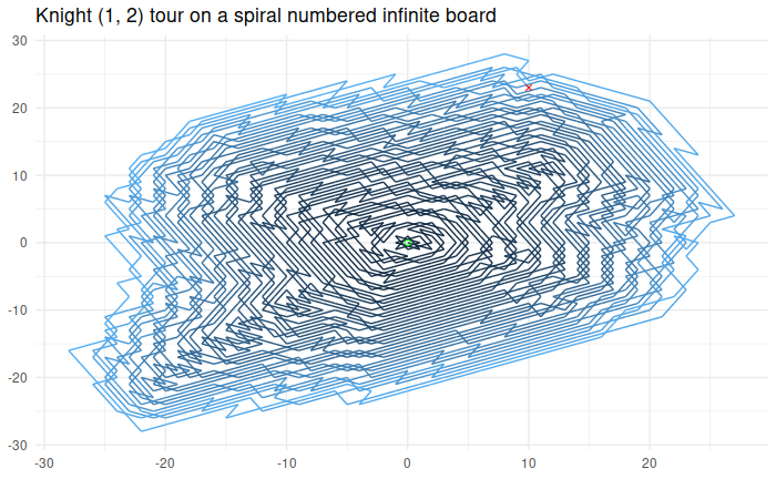
NumberPhile did a video on potentially infinite Knight Tours that I found quite interesting. I wanted to test out literate programming using Quarto to solve it and I did (result) 🙂
The RStudio integration with Quarto is really good and for a problem like this it really helps to keep your thoughts and code in the same place. Plots like this one that shows the complete tour are displayed inline and the experience is comparable with a Jupyter notebook with the advantage that it is not in the browser but in a polished IDE.
In my previous post I looked at the Tikz capabilities of ChatGPT. The quality of the graphics produced were above my expectations but I wouldn’t call them useful. While doing research for this interesting Quant.SE question I came up with a more interesting question. Can ChatGPT explain and plot option strategies? Turns out it can not but since I’m doing science on this blog, I share with you the results below anyways.
Maybe it can be coaxed into giving better results with better prompts. I’d be happy to hear if someone can. In any case, these were mine:
Please explain me some popular option trading strategies together with Tikz graphics For each of the graphics can you write Tikz code? Can you give me the Tikz code for a straddle, a strangle and iron condor as well
For some reason it got distracted when generating the graphs. The results are summarized below. Note again: this is all ChatGPT output, I only combined the graphics and compiled the Tikz.
Sure, I can explain some popular option trading strategies, but as a text-based AI, I’m unable to directly create Tikz graphics. However, I can certainly describe them in a way that can help you visualize and perhaps draw them yourself.
Long Call: This is the most basic options strategy. When you buy a call option, you’re buying the right to purchase a stock at a specified price (the strike price) before a specified date (the expiration date). You would use this strategy if you believe the price of the underlying asset is going to rise. Visualization: Imagine a graph with profit/loss on the Y-axis and the price of the underlying asset on the X-axis. The graph would be a diagonal line starting from the negative Y-axis (representing the premium paid for the call) and moving upward as the price of the underlying asset increases.
Long Put: This strategy involves buying a put option, which gives you the right to sell a stock at a specified price before a specified date. You would use this strategy if you believe the price of the underlying asset is going to fall. Visualization: The graph for a long put is a mirror image of the long call. It starts at the negative Y-axis (representing the premium paid) and moves downward as the price of the underlying asset increases.
Covered Call: This strategy involves owning the underlying asset and selling a call option on that asset. This is typically done when you believe the price of the asset will stay relatively stable, and you want to earn the premium from selling the call. Visualization: The graph starts at the Y-axis at the point where the premium for selling the call is added to the price of the asset. It then moves horizontally to the strike price of the call option, at which point it starts moving downward as the price of the asset increases.
Protective Put: This involves owning the underlying asset and buying a put option on that asset. This is done when you want to protect against a possible drop in the price of the asset. Visualization: The graph starts at the Y-axis at the point where the price of the asset is reduced by the premium for the put. It then moves horizontally to the strike price of the put option, at which point it starts moving upward as the price of the asset decreases.
Straddle: This strategy involves buying a call and a put option on the same asset with the same strike price and expiration date. This is typically done when you expect a big move in the price of the asset, but you’re not sure in which direction. Visualization: The graph for a straddle looks like a V, with the point of the V at the strike price of the options. The left side of the V represents the profit/loss for the put option and the right side represents the profit/loss for the call option.
Strangle: Similar to a straddle, but the call and put options have different strike prices. This is typically done when you expect a big move in the price of the asset, but you’re not sure in which direction, and you want to reduce the cost of the strategy by choosing strike prices that are out of the money. Visualization: The graph for a strangle looks similar to a straddle, but the V is wider due to the different strike prices.
Iron Condor: This is a more advanced strategy that involves selling a call spread and a put spread on the same asset. This is typically done when you expect the price of the asset to stay within a certain range. Visualization: The graph for an iron condor looks like a bird in flight, with the body of the bird representing the range within which you profit and
Just as the descriptions the graphics aren’t very good unfortunately. It seems to have to have difficulty with combining the different pay off structures of the parts of the strategy.
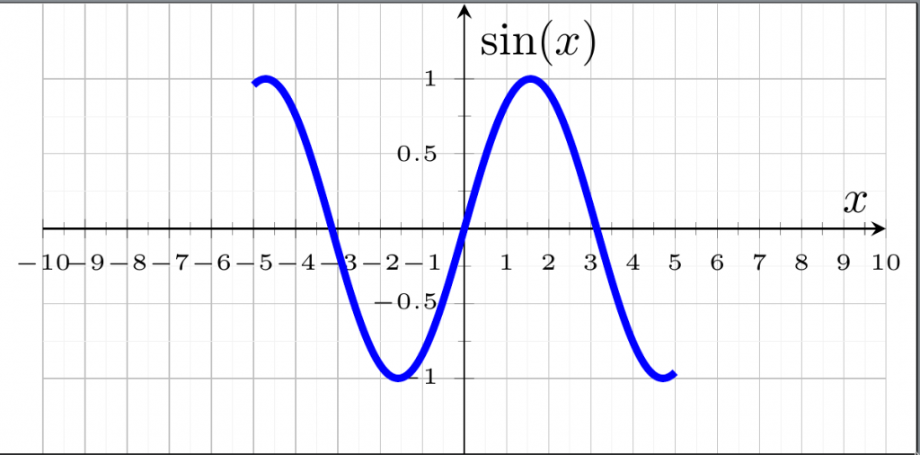
Sometime ago through HackerNews I found this experiment on drawing a unicorn with ChatGPT on the blog of Adam K Dean. The results left something to be desired. I prefer using Tikz instead of SVG so I decided to an experiment myself with reasonable results. First I wanted a simple sine wave. In 2014, during an interview, I was asked to sketch a sine wave on a whiteboard as a preliminary step for a problem the interviewers wanted me to tackle. Regrettably, I ended up poorly drawing a cosine wave instead. For ChatGPT however, it’s not a problem:
A rather detailed plot of a sine wave generated with the prompt: “Can you give me a sine wave plot with tikz”
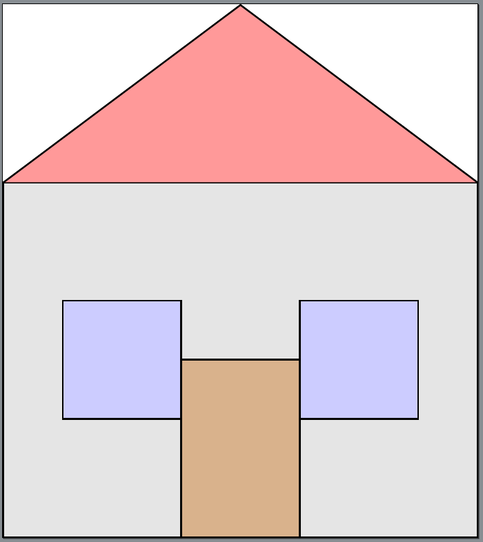
This is pretty good, I know I would need to some searching to get to this. Next I wanted a house:
A very simple house created with Tikz and the prompt: “Draw a house in Tikz”
This is going better than expected, let’s try to draw a unicorn:
A simple unicorn generated with prompt: “Draw a unicorn in Tikz”
Please add some details:
After prompt: “Please add some details”
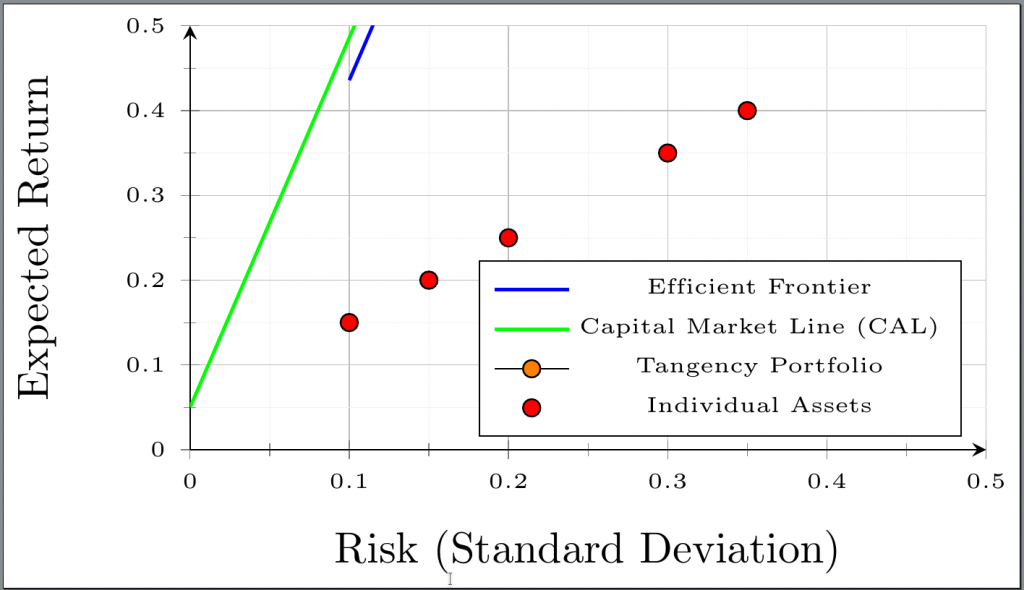
It does try hard to give me an Markowitz efficent frontier together with the Capital Allocation Line and the tangency portfolio but didn’t quite succeed. This is the final result of the prompts: “Now draw an Markowitz efficent frontier with some details”, “Can you add the CAL and the tangency portfolio?” and “Please don’t use path”. The latest command is necessary as my installation of Tikz doesn’t know about it but it appears to work in another version. The result isn’t great, by default the legend is over the points and I need to comment out the location of the tangency portfolio. That said, if one really wants to get this graph ChatGPT gives a great start and it writes around 40 lines of Tikz code in 2 minutes which I’m definitely not able to do.
A part of the efficient frontier with individual assets. The tangency portfolio has been commented out and the legend has been moved manually from ‘north west’ to south east.
where move_fun was either identity() or rev(). Getting the data into shape was more interesting and the native pipe could be put to good use as well as a new experminental feature:
The pipebind operator => in the middle of this pipeline can be used to the current argument to a name in the middle of a pipe. This allows using the current argument of the pipeline without the need to resort to ad hoc anonymous functions. Since it’s an experimental feature, it must be activated. This can be done by putting this in your .Rprofile: Sys.setenv("R_USE_PIPEBIND"=TRUE). This also works in RStudio.
Day 6
Day 6 was the easiest puzzle until now but I learned one small trick: The base function match() has an optional argument nomatch which specifies the return value if no match is found. In this case an if statement can be avoided by setting nomatch=0. The code below gets the part from a index to the end or keeps the buffer with one char added:
This puzzle gave a good reason to start the Dictionary class in recollections! Unlike the builtin list datatype the recollections dictionary can be used by reference which allowed finding a directory and directly using it without the need to copy it back into the directory tree. On top of that, the C++ code that underlies the Dictionary class is more efficient than that of list. With the tree of dictionaries in place, the logic to find the sizes of all leaves in the tree is a standard use of recursion.
Day 8
I’m not completely happy with this solution to this puzzle. After tinkering and looking at profvis output I managed to create a solution that runs in less than 10 seconds on this old machine but if the forest gets much bigger this code will struggle. Putting the puzzle input into a data.table might not be the most natural thing to do but in the end to write a quite clear solution so maybe it’s not all bad.
Day 9
In this puzzle we were asked to implement some weird version of snake. Again, this seems to be best solved using recollections::Dictionary to keep track of which cells have been visited. My initial solution solution had quite a bit of logic to determine the moves in the tail but this Reddit comment that simplified the logic quite a bit. Despite being a similar solution it’s interesting to see that the Python and R solution use quite different language features.
In this exercise it seems logical to put all properties of the individual monkeys in some kind of class. So, this was a good moment to play around with S4 classes. This worked out quite well but I did notice there is a bit of overhead when one interacts with the slots of the classes. By batching slot manipulation a speed of 50% was achieved. This performance improvement is unlikely to be relevant for most uses of R though as a lot of R code won’t have such tight loops.
This Advent period I’m participating in the Advent of Code (AoC) using R base + data.table and put the code on GitHub. Till now, the given data is easily be manipulated and there was even no need to use conditions or loops to get to the answers. Just using the functions in R base or loading and manipulating the data with data.table was sufficient thanks to tstrsplit(), and foverlaps().
CRAN automatically checks C/C++ source code packages for Undefined Behaviour (UB). If the automated checks find UB it might result in the removal of the package from CRAN. This is a good thing, the presence of UB is a potential source of bugs and has no positive side effects. These checks have been improving and found scrypt package actually had some UB which needed to be fixed. This scared me a bit since although I’m a maintainer since the package contains some relatively complicated code which I didn’t write or change. A bit of history: Colin Percival conceived and implemented the algorithm in C and Andrew Kipp ported his code to R. I only revived the package after improved automated checks found problems that needed to be solved.
Reproducing the issue was my first challenge. My machine runs Ubuntu LTS and doesn’t have all the fancy tools installed to detect the UB. If I’m not able to reproduce the issue I can’t know whether I fixed it either so reproducing seemed like a good first step. I asked on Twitter and Dirk Eddelbuettel pointed me to the repo of a Docker image purpose made for this kind of analysis by Winston Chang. The instructions are worth reading but this is all I needed:
docker run --rm -ti --security-opt seccomp=unconfined -v $(pwd):/rscrypt wch1/r-debug
This downloads the docker image if you don’t have it yet and starts it with the current directory mounted to /rscrypt inside the container. Within the container you can access versions of R with extra instrumentation. For detecting the UB two versions are available: RDsan (san is shorthand for sanitizer) which is compiled with gcc and RDcsan which is compiled with clang. So now I could do (some output elided):
R> RDcsan CMD INSTALL scrypt_0.1.3.tar.gz  # The last version with the problem
R> scrypt::hashPassword("password")
scrypt-1.1.6/lib/crypto/sha256.c:254:24: runtime error: null pointer passed as argument 2, which is declared to never be null
/usr/include/string.h:44:28: note: nonnull attribute specified here
    #0 0x7f21fe3bde7f in scrypt_SHA256_Update /tmp/.../sha256.c:254:3
    #1 0x7f21fe42b1e6 in scrypt_HMAC_SHA256_Update /tmp/.../sha256.c:335:2
    #2 0x7f21fe42b6a1 in PBKDF2_SHA256 /tmp/../sha256.c:377:2
    #3 0x7f21fe42c9e6 in crypto_scrypt /tmp/.../crypto_scrypt-ref.c:258:2
    #4 0x7f21fe46f822 in getcpuperf(double*) /tmp/.../util.cpp:145:13
    #5 0x7f21fe46420c in (anonymous namespace)::getparams(double, double, int*, unsigned int*, unsigned int*) /tmp/.../scrypt.cpp:49:15
    #6 0x7f21fe462f81 in hashPassword(std::__cxx11::basic_string<char, std::char_traits<char>, std::allocator<char> > const&, double, double) /tmp/.../scrypt.cpp:129:15
    #7 0x7f21fe439c72 in _scrypt_hashPassword /tmp/.../RcppExports.cpp:17:34
...
etc
The C code of the scrypt package is entered at #7.
The CRAN error report shows that UB was with R compiled by using both gcc and clang but for some reason when I tried the issue was only flagged by RDcsan. The important thing is the error can be reproduced and a possible fix can be validated.
In this particular case the error was easy to find. The code that triggers the UB is the following memcpy() and from the error message we know that the src argument is the culprit:
memcpy(&ctx->buf[r], src, len);
Tracing through the call stack I found that the src in this case is the salt used when figuring out how many iterations scrypt should perform to perform reasonably well on the current machine. More importantly, for this test the hash has the value NULL. This explains the error found: memcpy() can’t copy anything from NULL.
With the root cause identified, the solution is simple: set the initial salt to an actual value, since this code is only called when checking the CPU performance and since the old behaviour is UB anyway it doesn’t really make a difference what value is used. I choose to set it to all zeroes. After that, the UB disappeared, a commit was pushed and a submission to CRAN was accepted.
Lessons learned
CRAN has been checking packages for UB since 2014 and the checks are still improving, great!
Finding UB like this requires help from good tooling which isn’t as easily available as R and CRAN
Luckily, smart people have figured out a way to get this tooling on your computer in a few minutes
Once I knew were to look, the problem was easily solved